for loops

A for loop is a way to repeat the same steps several times. It’s useful when we want to do something over and over again, like simulate a random experiment.

The pattern looks like this:

for (i in 1:N) {
  do_something
}

• i is the loop variable. It takes the values 1, 2, 3, …, up to N.
• The code inside the { } is repeated once for each value of i.

Example: Counting sixes in 100 dice rolls

six_count <- 0  # start a counter

for (i in 1:100) {
  roll <- sample(1:6, size = 1)
  if (roll == 6) {
    six_count <- six_count + 1
  }
}

six_count

[1] 16

• The loop goes through i = 1, 2, ..., 100.
  
• Each time, it rolls a die and checks if it’s a six.
  
• If it is, it increments six_count by 1.
  
• At the end, six_count is the total number of sixes rolled in 100 trials.

Example: plotting many lines

In this explainer, we saw how to use the curve function to plot lines. If you want a plot with many lines, you can just call the curve function many times with the add = TRUE argument to layer things. In that explainer, we just hard-coded the multiple calls to curve. A for loop can clean that up:

curve(1*x^2, from = -5, to = 5, n = 500, col = "red", ylab = "")

for(a in 2:25){
  curve(a*x^2, from = -5, to = 5, n = 500, ylab = "", add = TRUE)
}

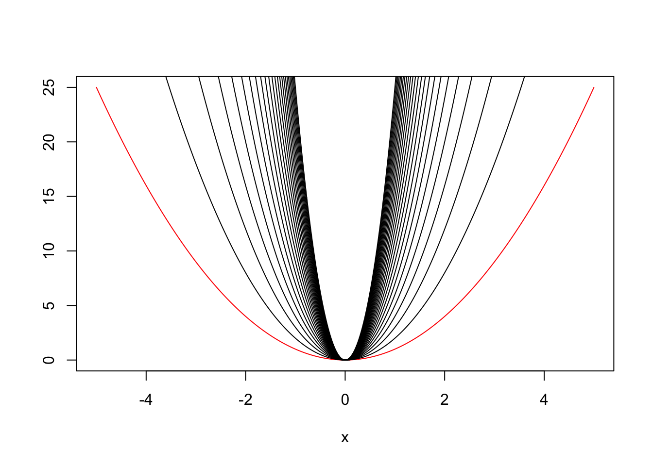
That code plots the function \(ax^2\) every value of \(a=1,\,2,\,3,\,...,\,25\). Instead of writing 25 calls to the curve function, I consolidate with a loop.