set.seed(152638)
U <- runif(5000)
X <- -log((1 / U) - 1)
hist(X, breaks = "Scott", freq = FALSE)
curve(exp(-x) / (1 + exp(-x))^2, from = min(X), to = max(X), n = 1000,
      col = "red", lwd = 2, add = TRUE)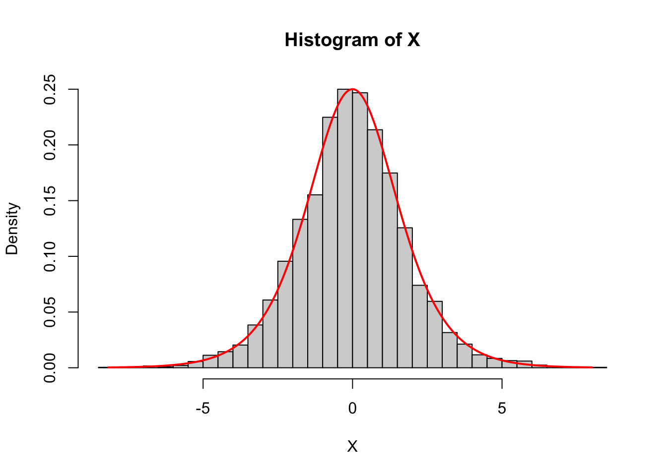
Due Thursday October 30 at 11:59 PM
When we call rnorm or rgamma or rpois to generate random numbers from one of our special distributions, what is the computer actually doing? How do we program a computer to generate random numbers that behave according to some pre-defined distribution?
At the end of the day, all simulation methods revolve around a simple principle: “simulate from the standard uniform and then apply a transformation.” We statisticians take from granted that the computer scientists have devised good methods for generating random numbers from Unif(0, 1). The Mersenne Twister is a popular algorithm. Given that we can generate random numbers from the standard uniform, we need to figure out how to transform them into a batch of new random numbers that follow the distribution we want: normal, gamma, Cauchy, whatever.
The following theorem is a proof of concept that “simulate Unif(0, 1) and transform” is sufficient, at least in theory, to simulate any distribution we can think of:
Let \(U\sim \text{Unif}(0,\, 1)\), and let \(F\) be any continuous cdf we are interested in. If we define a new random variable \(X=F^{-1}(U)\), then \(X\sim F\).
For simplicity, assume \(F\) is smooth and invertible. Things still work if it isn’t, but it makes the math a little cleaner. Furthermore, recall the cdf of the standard uniform \(U\sim\text{Unif}(0,\, 1)\): \[ F_U(x)=\begin{cases} 0 & x \leq 0\\ x & 0<x<1\\ 1 & 1 \leq x. \end{cases} \]
\(X\) is just a transformation of \(U\), so we can apply the cdf method. \[ \begin{align*} F_X(x) &= P(X\leq x) \\ &= P(F^{-1}(U)\leq x) \\ &= P(U\leq F(x)) \\ &= F_U\left(F(x)\right) \\ &= F(x) . \end{align*} \]
So, the cdf of \(X\) is literally just \(F\).
Now, in order to actually implement the algorithm, we need to be able to compute the inverse cdf \(F^{-1}\). In some cases, this may not be possible, and we must use a different transformation to actually get the job done. But the principle stands. Dig down deep enough into any simulation algorithm, and it’s just simulating uniforms and messing with them.
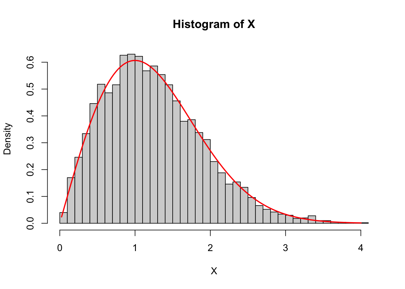
Consider a random variable \(X\) with this density:
\[ f(x) = \frac{e^{-x}}{(1+e^{-x})^2},\quad x\in\mathbb{R}. \]
n = 5000 random numbers from this distribution. Plot a histogram of the random numbers, and overlay a line plot of the original density function we gave you. If you did everything correctly, the histogram and the density should agree.This is the standard logistic distribution. The CDF is
\[ \begin{aligned} F(x) &= \int_{-\infty}^x f(t) dt \\ &= \int_{-\infty}^x \frac{e^{-t}}{(1+e^{-t})^2} dt \\ &= \int_{\infty}^{e^{-x}} \frac{-du}{(1+u)^2} &&\begin{matrix}u=e^{-t}\\ du = -e^{-t}dt\end{matrix} \\ &= \int_{e^{-x}}^{\infty} \frac{du}{(1+u)^2} \\ &= \left[-\frac{1}{1+t}\right]_{e^{-x}}^\infty \\ &= 0 - \left(-\frac{1}{1+e^{-x}}\right) \\ &= \frac{1}{1+e^{-x}},&&x\in\mathbb{R}. \end{aligned} \]
Inverting it gives
\[ \begin{aligned} u &= \frac{1}{1+e^{-x}}\\ 1+e^{-x} &= \frac{1}{u}\\ e^{-x} & = \frac{1}{u} - 1\\ -x &= \ln\left(\frac{1}{u} - 1\right)\\ x &= -\ln\left(\frac{1}{u} - 1\right). \end{aligned} \]
So the inverse CDF is
\[ F^{-1}(u)=-\ln\left(\frac{1}{u}-1\right),\quad 0<u<1. \]
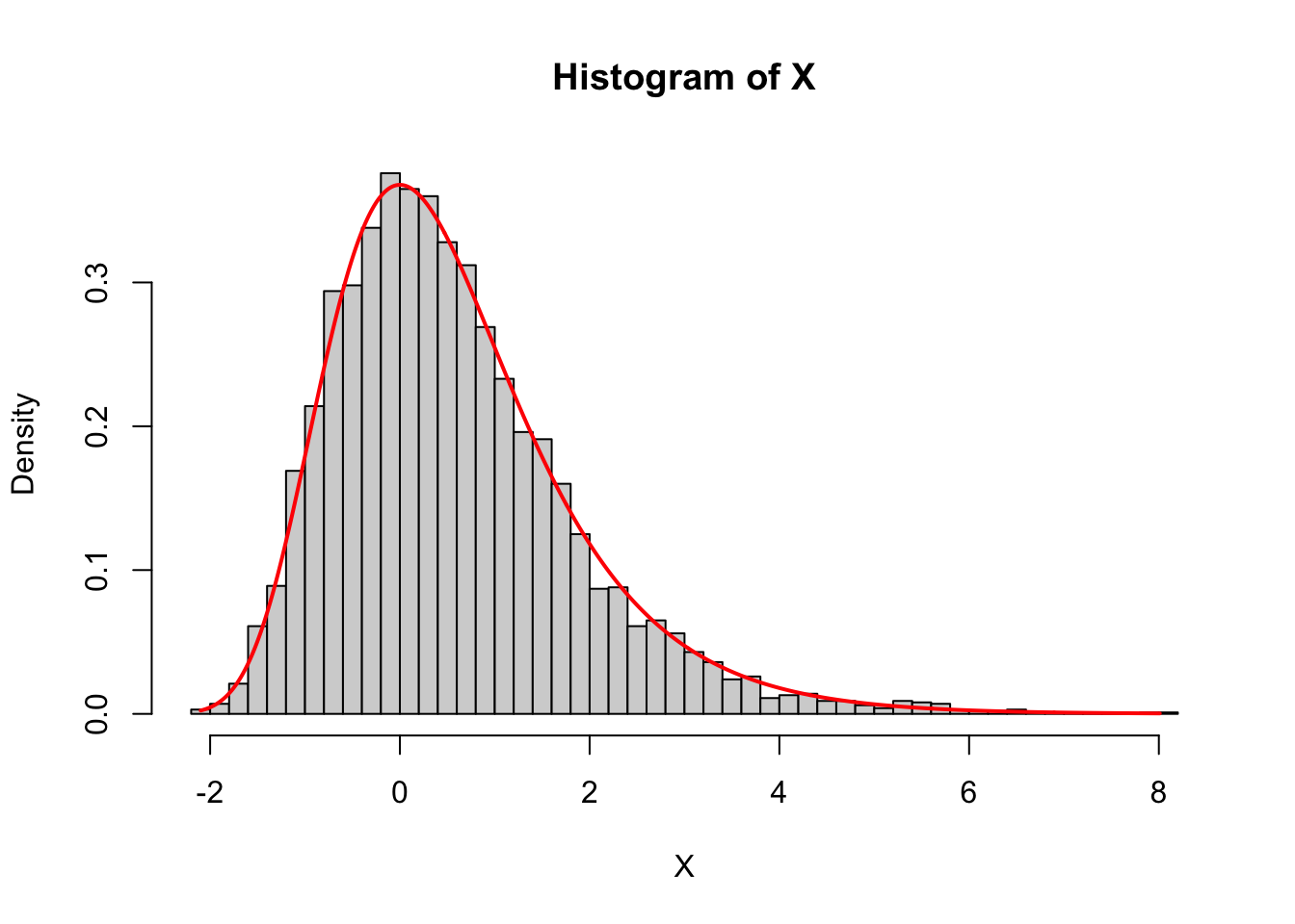
Consider a random variable \(X\) with this density:
\[ f(x) = xe^{-\frac{1}{2}x^2},\quad x\geq 0. \]
n = 5000 random numbers from this distribution. Plot a histogram of the random numbers, and overlay a line plot of the original density function we gave you. If you did everything correctly, the histogram and the density should agree.This is the Rayleigh distribution.
\[ \begin{aligned} F(x) &= \int_{-\infty}^x f(t) dt \\ &= \int_{0}^x te^{-\frac{1}{2}t^2} dt \\ &= \int_{0}^{-x^2/2} -e^u\,du && \begin{matrix} u=-t^2/2\\ du=-t\,dt \end{matrix} \\ &= \int_{-x^2/2}^0 e^u\,du \\ &= [e^u]_{-x^2/2}^0 \\ &= 1-e^{-x^2/2},&&x\geq 0. \end{aligned} \]
Invert it:
\[ \begin{aligned} u &= 1-e^{-x^2/2}\\ e^{-x^2/2} &= 1 - u\\ -x^2/2&=\ln(1-u)\\ x^2&=-2\ln(1-u)\\ x&=\sqrt{-2\ln(1-u)} \end{aligned} \]
So
\[ F^{-1}(u)=\sqrt{-2\ln(1-u)}, \quad 0<u<1. \]
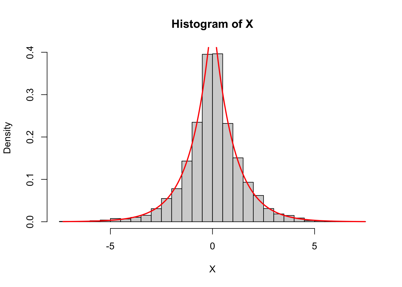
Consider a random variable \(X\) with this density:
\[ f(x) = e^{-(x+e^{-x})},\quad x\in\mathbb{R}. \]
n = 5000 random numbers from this distribution. Plot a histogram of the random numbers, and overlay a line plot of the original density function we gave you. If you did everything correctly, the histogram and the density should agree.This is the standard Gumbel distribution.
\[ \begin{aligned} F(x) &= \int_{-\infty}^x f(t) dt \\ &= \int_{-\infty}^x e^{-(t+e^{-t})} dt \\ &= \int_{\infty}^{e^{-x}} -e^{-(-\ln u+u)} \frac{du}{u} && \begin{matrix} u=e^{-t}\\ du=-e^{-t}\,dt \end{matrix} \\ &= \int_{e^{-x}}^\infty e^{-u}du \\ &= [-e^{-u}]_{e^{-x}}^\infty \\ &= 0-(-e^{-e^{-x}}) \\ &= e^{-e^{-x}},&& x\in\mathbb{R}. \end{aligned} \]
Invert it:
\[ \begin{aligned} u &= e^{-e^{-x}}\\ \ln u&=-e^{-x}\\ -\ln u &=e^{-x}\\ \ln(-\ln u)&=-x\\ -\ln(-\ln u)&=x. \end{aligned} \]
So
\[ F^{-1}(u)=-\ln(-\ln u),\quad 0<u<1. \]
Consider a random variable \(X\) with this density:
\[ f(x) = \frac{1}{2}e^{-|x|},\quad x\in\mathbb{R}. \]
n = 5000 random numbers from this distribution. Plot a histogram of the random numbers, and overlay a line plot of the original density function we gave you. If you did everything correctly, the histogram and the density should agree.This is the standard Laplace distribution. For \(x<0\),
\[ \begin{aligned} F(x) &= \int_{-\infty}^x \frac{1}{2}e^{-|t|}\,\text{d}t \\ &= \frac{1}{2} \int_{-\infty}^x e^{-(-t)}\,\text{d}t \\ &= \frac{1}{2} \int_{-\infty}^x e^{t}\,\text{d}t \\ &= \frac{1}{2} [e^t]_{-\infty}^x \\ &= \frac{1}{2} e^x. \end{aligned} \]
For \(x\geq 0\),
\[ \begin{aligned} F(x)&=P(X\leq x) \\ &=1-P(X>x) \\ &=1-\int_x^\infty \frac{1}{2}e^{-|t|}\,\text{d}t \\ &= 1-\frac{1}{2}\int_x^\infty e^{-t}\,\text{d}t \\ &= 1-\frac{1}{2}[-e^{-t}]_x^\infty \\ &= 1-\frac{1}{2}e^{-x}. \end{aligned} \]
So
\[ \begin{aligned} F(x) &= \begin{cases} \frac{1}{2} e^x & x<0\\ 1-\frac{1}{2} e^{-x} & x\geq 0. \end{cases} \end{aligned} \]
If you invert that darn thing, you get:
\[ \begin{aligned} F^{-1}(u)=\text{sign}(u-0.5)\ln(1-2|u-0.5|),\quad 0<u<1. \end{aligned} \]
I love computer simulation. It’s gorgeous. Here are two great books: