set.seed(2345)
n <- 100
theta <- 4
X <- sqrt(-2 * theta * log(1 - runif(n)))
hist(X, breaks = "Scott", freq = FALSE)
curve(exp(-x^2/(2*theta)) * x / theta,
      from = 0, to = max(X), n = 1000, col = "red", add = TRUE)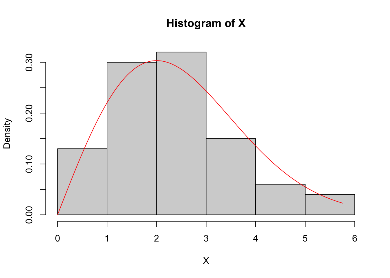
Due Thursday November 20 at 11:59 PM
This lab provides extra practice with the kind of maximum likehood problem that you will encounter on the last problem set and the final exam.
If a non-negative random variable \(X\) has the Rayleigh distribution with parameter \(\theta>0\), then its CDF is
\[ F(x;\,\theta)=1-\exp\left(-\frac{x^2}{2\theta}\right)\quad x\geq 0, \]
and we say \(X\sim\text{Rayleigh}(\theta)\). What is the PDF in this parametric family?
\[ \begin{aligned} f(x;\,\theta) &= F'(x;\,\theta) \\ &= \frac{\text{d}}{\text{d}x} \left[ 1-\exp\left(-\frac{x^2}{2\theta}\right) \right] \\ &= 0-\frac{-x}{\theta} \exp\left(-\frac{x^2}{2\theta}\right) \\ &= \frac{x}{\theta} \exp\left(-\frac{x^2}{2\theta}\right),&&x\geq 0. \end{aligned} \]
Imagine we observe data
\[ X_1,\,X_2,\,...,\,X_n\overset{\text{iid}}{\sim}\text{Rayleigh}(\theta), \]
where the true value of the parameter \(\theta>0\) is unknown. Use the method of maximum likelihood to propose an estimator for \(\theta\).
The likelihood function is
\[ \begin{aligned} L(\theta;\,X_{1:n}) &= \prod_{i=1}^n f(X_i;\,\theta) \\ &= \prod_{i=1}^n \frac{X_i}{\theta} \exp\left(-\frac{X_i^2}{2\theta}\right) \\ &= \theta^{-n}\left(\prod_{i=1}^nX_i\right)\left[\prod_{i=1}^n\exp\left(-\frac{X_i^2}{2\theta}\right)\right] \\ &= \theta^{-n}\left(\prod_{i=1}^nX_i\right)\exp\left(-\frac{1}{2\theta}\sum\limits_{i=1}^nX_i^2\right). \end{aligned} \]
The log-likelihood function is
\[ \begin{aligned} \ell(\theta;\,X_{1:n}) &= \ln L(\theta;\,X_{1:n}) \\ &= \ln\left[\theta^{-n}\left(\prod_{i=1}^nX_i\right)\exp\left(-\frac{1}{2\theta}\sum\limits_{i=1}^nX_i^2\right)\right] \\ &= \ln(\theta^{-n})+\ln\left(\prod_{i=1}^nX_i\right)+\ln\left[\exp\left(-\frac{1}{2\theta}\sum\limits_{i=1}^nX_i^2\right)\right] \\ &= -n\ln \theta+\sum\limits_{i=1}^n\ln X_i-\frac{1}{2\theta}\sum\limits_{i=1}^nX_i^2 . \end{aligned} \]
To maximize this, we take the second derivative, set it equal to zero, and solve:
\[ \begin{aligned} \frac{\text{d}}{\text{d}\theta}\ell(\theta;\,X_{1:n}) = - \frac{n}{\theta} + \frac{1}{2\theta^2} \sum\limits_{i=1}^nX_i^2 &= 0 \\ \frac{1}{2\theta^2} \sum\limits_{i=1}^nX_i^2 &= \frac{n}{\theta} \\ \frac{1}{2n} \sum\limits_{i=1}^nX_i^2 &= \theta. \end{aligned} \]
So the maximum likelihood estimator for the Rayleigh distribution is
\[ \hat{\theta}_n=\frac{1}{2n} \sum\limits_{i=1}^nX_i^2. \]
Your estimator in the previous part is a random variable that inherits its randomness from the \(X_i\). Derive the full sampling distribution of your estimator.
For these problems, I work “from the inside out.” What’s the distribution of \(X_i\)? What’s the distribution of \(X_i^2\)? What’s the distribution when you add those up? What’s the distribution when you scale the sum by \(1/2n\)? To answer those questions, you need tools like the change-of-variables formulas and our MGF updating rules for linear combinations.
We already know that \(X_1\sim\text{Rayleigh}(\theta)\), so we derive the distribution of \(Y_1=g(X_1)=X_1^2\) using change of variables. Since \(\text{Range}(X_1)=(0,\,\infty)\), the transformation is strictly increasing, so we apply the change of variables formula:
\[ \begin{aligned} f_{Y_1}(y) &= f\left(g^{-1}(y);\,\theta\right)\left|\frac{\text{d}}{\text{d}y}g^{-1}(y)\right| \\ &= f\left(y^{1/2};\,\theta\right)\left|\frac{\text{d}}{\text{d}y}y^{1/2}\right| \\ &= \frac{y^{1/2}}{\theta} \exp\left(-\frac{(y^{1/2})^2}{2\theta}\right) \left|\frac{1}{2}y^{-1/2}\right| \\ &= \frac{y^{1/2}y^{-1/2}}{2\theta} \exp\left(-\frac{y}{2\theta}\right) \\ &= \frac{1}{2\theta} \exp\left(-\frac{y}{2\theta}\right) ,&&y>0. \end{aligned} \]
This is the density of \(\text{Exponential}(1/2\theta)\), otherwise known as \(\text{Gamma}(1,\,1/2\theta)\). Given this, we have the following:
\[ \begin{aligned} X_i\overset{\text{iid}}{\sim}\text{Rayleigh}(\theta) \quad &\implies \quad X_i^2\overset{\text{iid}}{\sim}\text{Gamma}(1,\,1/2\theta) \\ &\implies \sum\limits_{i=1}^nX_i^2\sim\text{Gamma}(n,\,1/2\theta) \\ &\implies \frac{1}{2n}\sum\limits_{i=1}^nX_i^2\sim\text{Gamma}(n,\,n/\theta). \end{aligned} \] The last implication follows from Problem Set 5 #10d. So, the full sampling distribution of the estimator is
\[ \hat{\theta}_n\sim \text{Gamma}(n,\,n/\theta). \]
Now that you know the sampling distribution of the estimator, compute its mean squared error (MSE) using the bias-variance decomposition. Is the estimator unbiased? Is it consistent?
Using the mean and variance formulas for the gamma distribution, we see that
\[ \begin{aligned} E(\hat{\theta}_n)&=\frac{n}{n/\theta}=\theta\\ \text{var}(\hat{\theta}_n)&=\frac{n}{(n/\theta)^2}=\frac{\theta^2}{n}. \end{aligned} \]
Since \(E(\hat{\theta}_n)=\theta\), the bias of the estimator is zero, and so the mean-squared-error is simply \(\text{var}(\hat{\theta}_n)=\theta^2/n\). As \(n\to\infty\), this goes to zero. As such, the estimator is unbiased and consistent.
Compute the quantile function of the Rayleigh distribution and use it to generate 100 draws from the distribution that has \(\theta=4\).
The quantile function is the inverse cdf, so we solve:
\[ \begin{aligned} y &= 1-\exp\left(-\frac{x^2}{2\theta}\right) \\ \exp\left(-\frac{x^2}{2\theta}\right) &= 1-y \\ -\frac{x^2}{2\theta} &= \ln(1-y) \\ x^2 &= -2\theta\ln(1-y) \\ x &= \sqrt{-2\theta\ln(1-y)} . \end{aligned} \]
So \(F^{-1}(y;\,\theta)=\sqrt{-2\theta\ln(1-y)}\). As such, we can implement an inverse transform sampler to simulate from the distribution:
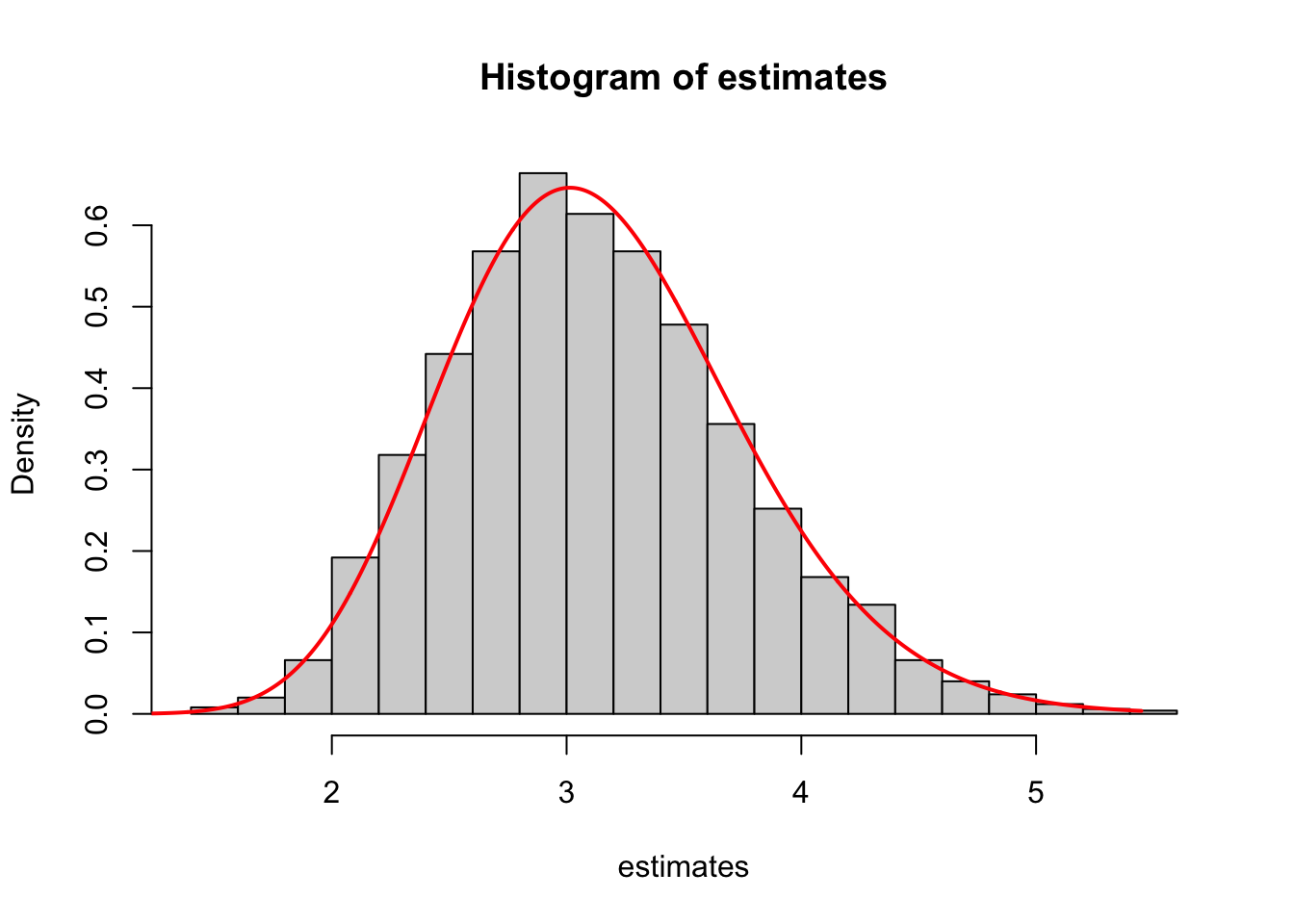
Write a for loop that simulates the sampling distribution for your estimator. Here is a schematic of what you are doing:
\[ \begin{matrix} \text{0. True parameter value} &&& \theta_0 && \\ &&& \downarrow && \\ \text{1. True distribution} &&& \text{Rayleigh}(\theta_0) && \\ &\swarrow &\swarrow& \cdots &\searrow&\searrow \\ \text{3. Simulated data}&x_{1:n}^{(1)} &x_{1:n}^{(2)}& \cdots &x_{1:n}^{(M-1)}&x_{1:n}^{(M)} \\ &\downarrow &\downarrow& \cdots &\downarrow&\downarrow \\ \text{4. Different estimates}&\hat{\theta}_n^{(1)} &\hat{\theta}_n^{(2)}& \cdots &\hat{\theta}_n^{(M-1)}&\hat{\theta}_n^{(M)} \\ &\searrow &\searrow& \cdots &\swarrow&\swarrow \\ & && \text{Histogram} && \\ \end{matrix} \]
At the end, add on top of the histogram a curve of the density that you derived in Task 3. They ought to match.
Here is some template code you can fill in:
true_theta <- 3.14      # true value of parameter
n <- 25                 # sample size
M <- 2500               # how many repetitions
estimates <- numeric(M) # preallocate storage for the sample of estimates

for(m in 1:M){
  # Step 1: simulate a new fake dataset of size n
  # Step 2: apply your formula from Task 2 to compute new estimate
  # Step 3: store it
}

# Step 4: plot histogram of estimates
# Step 5: add density curve of exact sampling distributionset.seed(123)
true_theta <- 3.14 # true value of parameter
n <- 25 # sample size
M <- 2500 # how many repetitions
estimates <- numeric(M) # preallocate storage for the sample of estimates
for(m in 1:M){
X <- sqrt(-2 * true_theta * log(1 - runif(n)))
estimates[m] <- sum(X^2) / (2*n)
}
hist(estimates, breaks = "Scott", freq = FALSE)
curve(dgamma(x, shape = n, rate = n / true_theta),
from = 0, to = max(estimates), n = 1000, col = "red",
lwd = 2, add = TRUE)