Lab 6

Due Thursday October 16 at 11:59 PM

In this lab you will get some basic practice with the tools R provides for working with special families of (absolutely) continuous random variables. Fortunately, these are the same tools you saw for discrete random variables in Lab 5: the p-, d-, r- functions.

The normal distribution

Imagine you are a theater producer. Your most recent smash hit was the musical Quiet!, a light, frothy adaptation of All Quiet on the Western Front. Your next project is a co-production with the Duke University Department of Statistical Science. It’s called Tidy!, and it features such rollicking numbers as “pivot the Night Away” and “facet_wrapped in Your Love.”

Let \(X\) represent the return-on-investment (ROI) for this new musical, which you can think of as ROI = (GAIN - INVESTMENT) / INVESTMENT. As I learned from this recent article in Significance magazine, investing in musicals is a risky business. You could make a killing, or you could lose your shirt. If \(X=0\), you broke even. If \(X>0\) you made money, and you have a hit if \(X\) is huge. If \(X<0\) you lost money, and if you used any debt or leverage in your financing, then \(X\) could be arbitrarily large in the wrong direction. All of these are possible. Furthermore, \(X\) is a proportion of money, and its value is uncertain. As such, it may be appropriate to model \(X\) as a continuous random variable that can take on any value in \(\mathbb{R}\).

By far the most famous model for such a variable is the normal distribution. Its density is the familiar bell curve, which you can play around with in this explainer. In what follows, imagine that \(X\sim\text{N}(\mu,\,\sigma^2)\), and historical experience tells us that returns are 0.1 (10%) on average with a standard deviation of 0.3.

Task 1

What is the probability that \(X\) will be exactly equal to 0.377?

Solution

This is a continuous random variable, so \(P(X=0.377)=0\).

Task 2

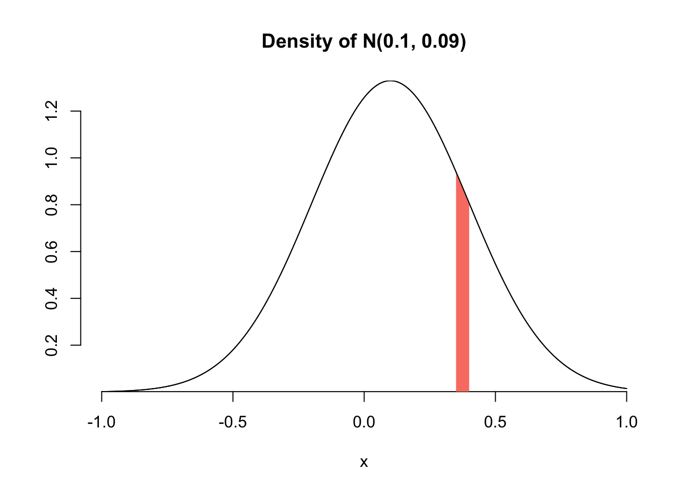
What is the probability that \(X\) will be somewhere between 0.35 and 0.4?

Solution

\(P(0.35<X<0.4)=F(0.4)-F(0.35)\):

pnorm(0.4, 0.1, 0.3) - pnorm(0.35, 0.1, 0.3)

[1] 0.04367313

This is the area of the shaded region under the density curve:

Task 3

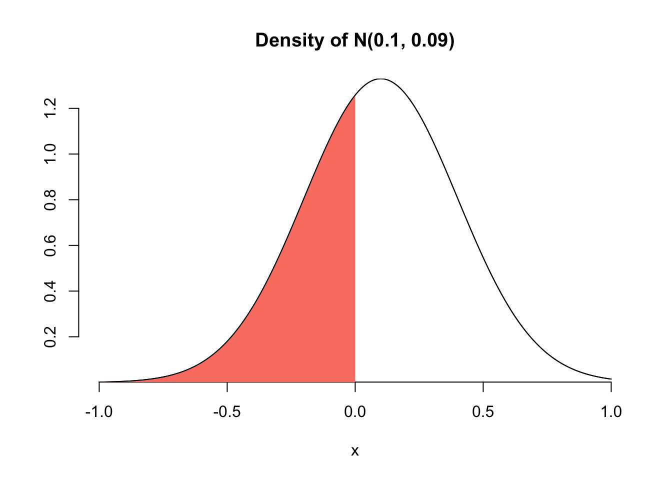
What is the probability that \(X\) will be negative?

Solution

\(P(X<0)=F(0)\):

pnorm(0, 0.1, 0.3)

[1] 0.3694413

This is the area of the shaded region under the density curve:

Task 4

Simulate n = 5000 realizations of \(X\) and then verify that the sample mean, the sample standard deviation, and the sample proportion of negative values agree with the “true,” theoretical numbers.

Set a seed!

To ensure that your numbers are reproducible and you get the same results every time you render your document, set a random number seed of your choosing.

Solution

set.seed(1234)
n <- 5000
x <- rnorm(n, 0.1, 0.3)

mean(x) # should be close to 0.1

[1] 0.09809359

sd(x) # should be close to 0.3

[1] 0.2974035

mean(x <= 0) # should be close to answer from Task 3

[1] 0.3684

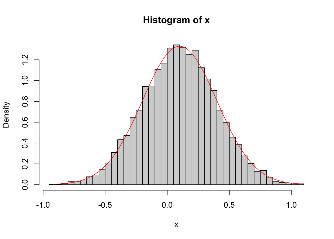
Task 5

Plot a histogram of your random numbers from the previous part, and overlay a line plot of the “true” density.

Solution

hist(x, breaks = "Scott", freq = FALSE)
curve(dnorm(x, mean = 0.1, sd = 0.3), 
      from = min(x), to = max(x), n = 1000, add = TRUE, col = "red")

The gamma distribution

Figure 1

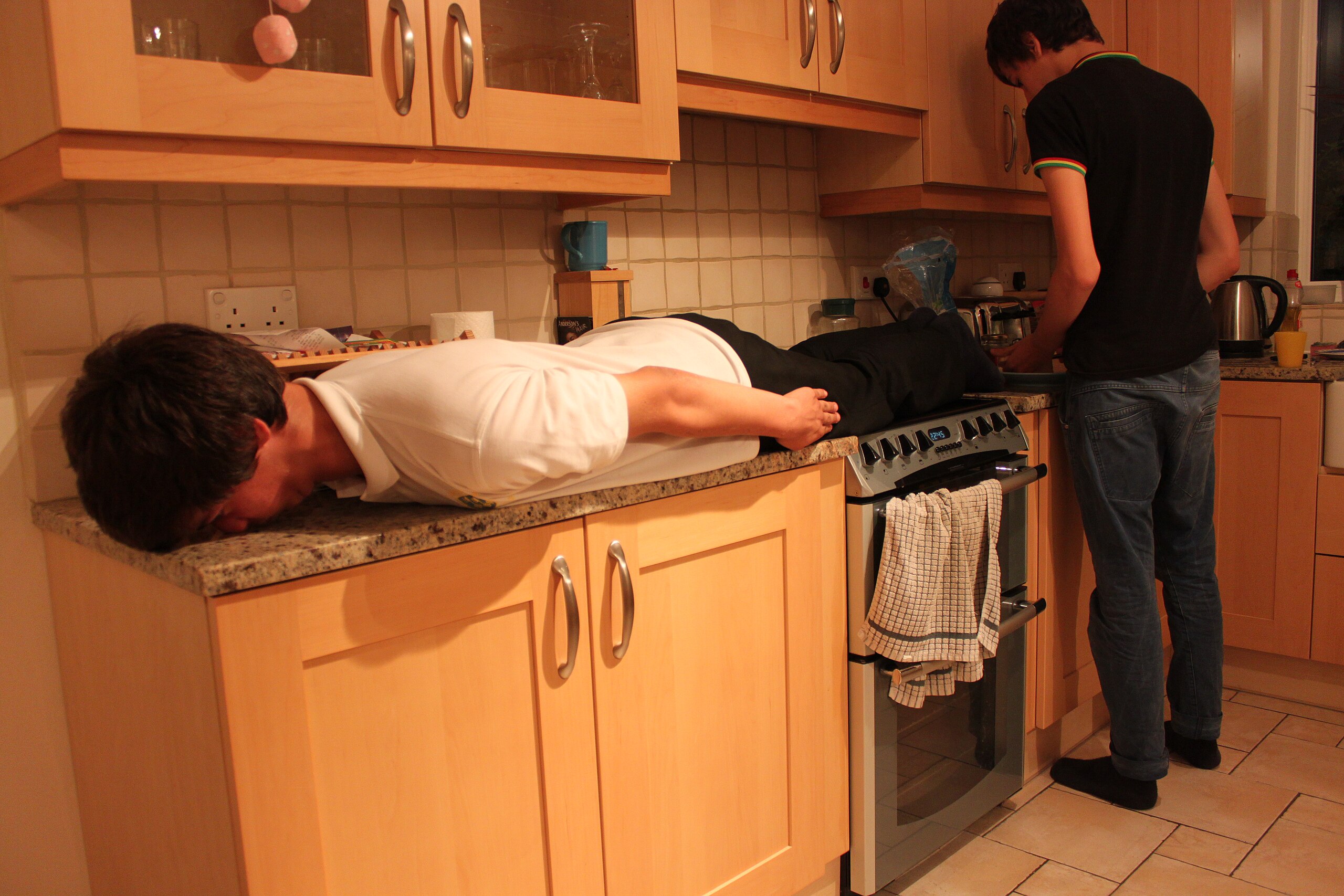
When I was in high school (2008 - 2012), a ridiculous fad emerged called “planking,” where people would photograph themselves in weird locations lying face down and stiff-as-a-board, as in Figure 1. It was really stupid. In a few sad cases, people chose to do this from great heights and accidentally plummeted to their deaths.

In addition to being a theater producer, imagine that you also own an insurance company that specializes in planking-related injuries. Every month, people submit claims against their policies for some amount of money. Let \(X\) represent the total dollar amount that your clients claim next month. This is a random variable because insurance claims are the result of random accidents. \(X\) is measured in units of dollars and cents, so it is most appropriate to model \(X\) as a continuous random variable that only takes on positive values.

A common model for such a variable is the gamma distribution, which has density:

\[ f(x) = \begin{cases} \frac{\beta^\alpha}{\Gamma(\alpha)}x^{\alpha-1}e^{-\beta x} &x\geq 0\\ 0 & x<0. \end{cases} \]

A random variable possessing this distribution is denoted \(X\sim\text{Gamma}(\alpha,\,\beta)\), and the parameters \(\alpha>0\) and \(\beta>0\) are called the shape and the rate. Once we have the appropriate tools, we will derive that \(E(X)=\alpha/\beta\) and \(\text{var}(X)=\alpha/\beta^2\), but for now you can just take these as facts. Our webpage has an explainer with more.

Task 6

The actuaries at your insurance company know that historically, monthly claims are about $10,000 on average, with a standard deviation of $2,000. If we want to use the model \(X\sim\text{Gamma}(\alpha,\,\beta)\), how should we set \(\alpha\) and \(\beta\) so that \(X\) has the correct location and spread?

Solution

We need \(\alpha/\beta = 10000\) and \(\sqrt{\alpha}/\beta=2000\). Alternatively, we need

\[ \frac{\alpha/\beta}{\sqrt{\alpha}/\beta}=\frac{10000}{2000}\,\implies\,\sqrt{\alpha}=5. \]

So \(\alpha = 5^2=25\). Consequently:

\[ \frac{25}{\beta}=10000\,\implies\,\beta=\frac{25}{10000}=0.0025. \]

Final answer: \(\alpha = 25\) and \(\beta = 0.0025\).

Task 7

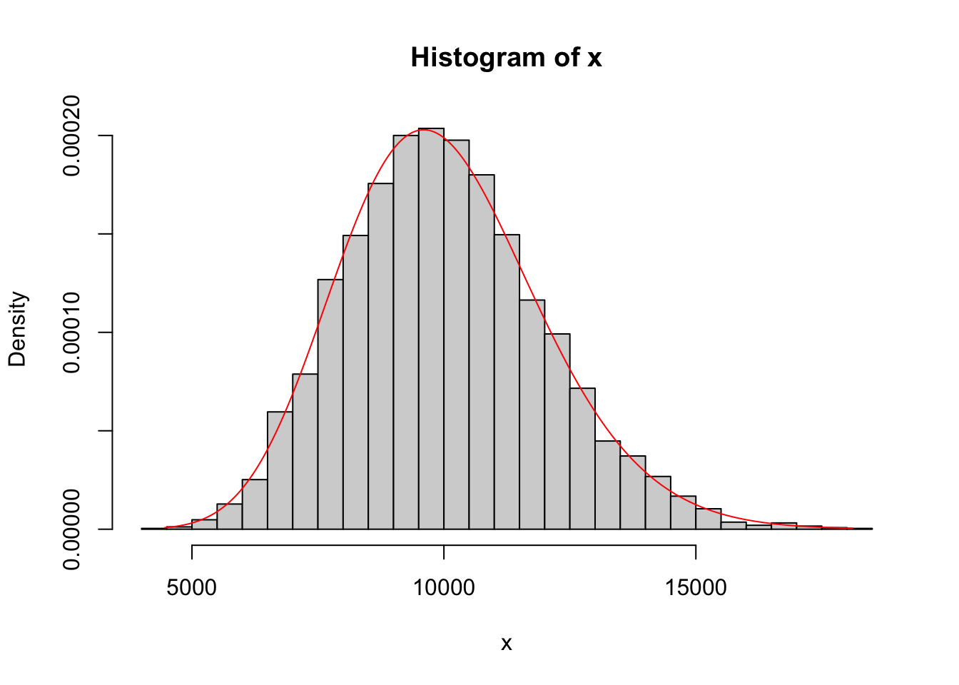
Simulate n = 5000 random numbers from the gamma distribution using the appropriate r- function. Plot a histogram of these numbers using the hist function, and overlay a line plot of the density using the curve function and the appropriate d- function.

Solution

set.seed(1234)
n <- 5000
x <- rgamma(n, 25, rate = 0.0025)
hist(x, breaks = "Scott", freq = FALSE)
curve(dgamma(x, 25, rate = 0.0025), 
      from = min(x), to = max(x), n = 1000, add = TRUE, col = "red")

Task 8

Verify that the sample mean and sample variance of your random numbers are close to the prescriptions from Task 6. If they are not, revisit Task 6 and adjust your choice of \(\alpha\) and \(\beta\) until this works.

Solution

mean(x) # should be close to 10000

[1] 10022.66

sd(x) # should be close to 2000

[1] 1972.818

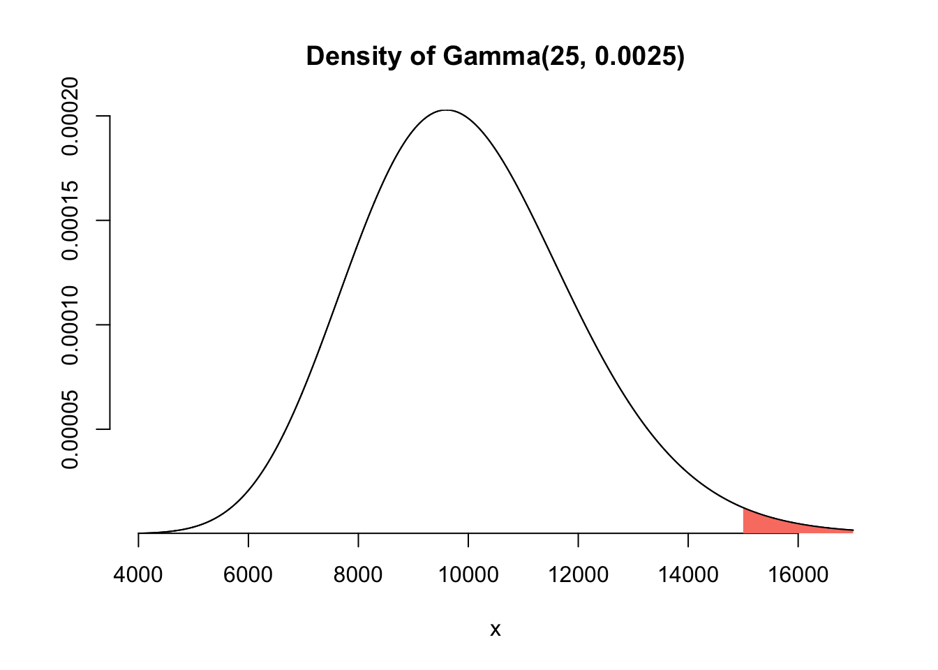
Task 9

What is the probability \(P(X > 15,000)\)? Calculate this probability exactly using the appropriate p- function, and also approximate it using your random numbers. Verify that the two numbers are close.

Solution

1 - pgamma(15000, 25, rate = 0.0025)

[1] 0.01259674

mean(x > 15000)

[1] 0.011

This is the area of the shaded region under the density curve: