[1] 0.01627706Lab 5
Due Thursday October 2 at 11:59 PM
Dating apps are horrific. Hopefully young people in college do not feel the need to use them. But for us decrepit old hags that were foolish enough to defer adulthood to the autumn of their thirties, they can feel unavoidable. So how do these work? Whelp, I make a profile, someone else on the app reviews it for no more than three seconds, and if I meet enough of their criteria, they swipe right (like my profile). If I fail to meet their criteria, they swipe left. If we both like each other’s profiles, it’s a match. God help us.
Let’s model this. When the other person reviews my profile, they are deciding if I possess qualities they value. What might those qualities be? Charm, humor, wealth, height, education, hygiene, style, a deep and abiding appreciation for the films of Luis Buñuel, etc. Figure 1 imagines that the set of potentially desirable qualities are balls in the proverbial urn. For the purposes of discussion, let’s say there are a total of one hundred qualities a person could potentially value (100 balls in the jar). Every human has a list of 8 that they care most about. Everyone’s different, so we will model a given person’s preferences as a random selection (without replacement!) of 8 balls from this jar of 100.
So, given a person’s preferences, will they like my profile? Well, let’s say that I possess exactly three of the one hundred desirable qualities. I won’t tell you what those three are, but suffice it to say, we have yet to list them in Figure 1. We will treat my three qualities as three red balls in the jar, and the remaining 97 are black. Next, let \(A\) be the event that at least two of my qualities are among the eight that a person values. If this happens, then they will swipe right on my profile.

Today’s goals
The main skills you will practice today are plotting PMFs and computing probabilities in our special families of discrete probability distributions. You may find these new explainers helpful:
Task 1
Imagine a random person on the app is presented with my profile. They will either like my profile and swipe right (1) or they won’t like it and they will swipe left (0). Define an indicator random variable \(I\) for this event:
\[ I =\begin{cases} 0 & \text{if $A^c$ happens} \\ 1 & \text{if $A$ happens}. \\ \end{cases} \]
What is the probability that a random person on the app swipes right on my profile? In other words, what is \(P(I=1)\)?
Solution
\[ \begin{aligned} P(I=1)=P(A)&=1-P(A^c)\\ &=1-P(\text{they value none or only one of my qualities})\\ &=1-P(\text{none})-P(\text{only one})\\ &=1-\frac{\binom{97}{8}}{\binom{100}{8}}-\frac{\binom{3}{1}\binom{97}{7}}{\binom{100}{8}}\\ &\approx 1 - 0.777 - 0.207\\ &=0.016. \end{aligned} \]
Task 2
Task 1 gives the probability that one person likes my profile, but as we all know, dating apps are a numbers game. One strategy is to go on there, indiscriminately swipe right on everyone until you run out of people in your area, wait for the matches to roll in, and then filter through only those folks that have already expressed interest in you. The dating app creators know this is a possibility though, and so they cap the number of right swipes you can send in a 24 hour period (unless you buy a premium subscription). Let’s say that number is \(n=25\), as I believe it is on Bumble. So on a given day, I send 25 likes out into the world. How many of those \(n=25\) people will like me back, resulting in a match? Introduce a binary random variable \(I_i\) indicating whether or not person \(i=1,\,2,\, ...,\,25\) likes my profile. Assume that these are all identically distributed as in Task 1, and assume that these are independent. We have yet to formally define this, but in context it means that the swiping decisions among these 25 people are not affecting one another. So none of them are sitting next to each other discussing my profile, for example.
Given this setup, define a new random variable \(X\) that counts the total number of matches I get. How is \(X\) related to the \(I_i\)? What is the distribution of \(X\)? What is \(E(X)\), the number of matches I expect to receive that day?
Solution
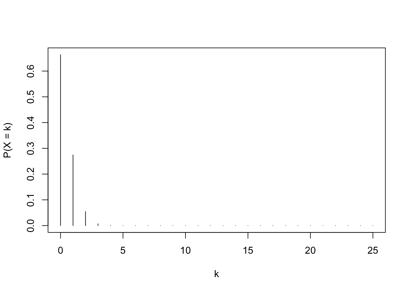
- \(X\sim\text{Binom}(25, 0.016)\);
- \(X=\sum_{i=1}^{25}I_i\);
- \(E(X) \approx 25\times0.016=0.4\).
Task 3
Use R to compute the probability that I get at least one match that day.
Solution
We want \(P(X\geq 1)=1-P(X=0)\):
match_prob <- 1 - dbinom(0, 25, like_prob)
match_prob
[1] 0.3365319Task 4
Use R to plot the PMF of \(X\).
Task 5
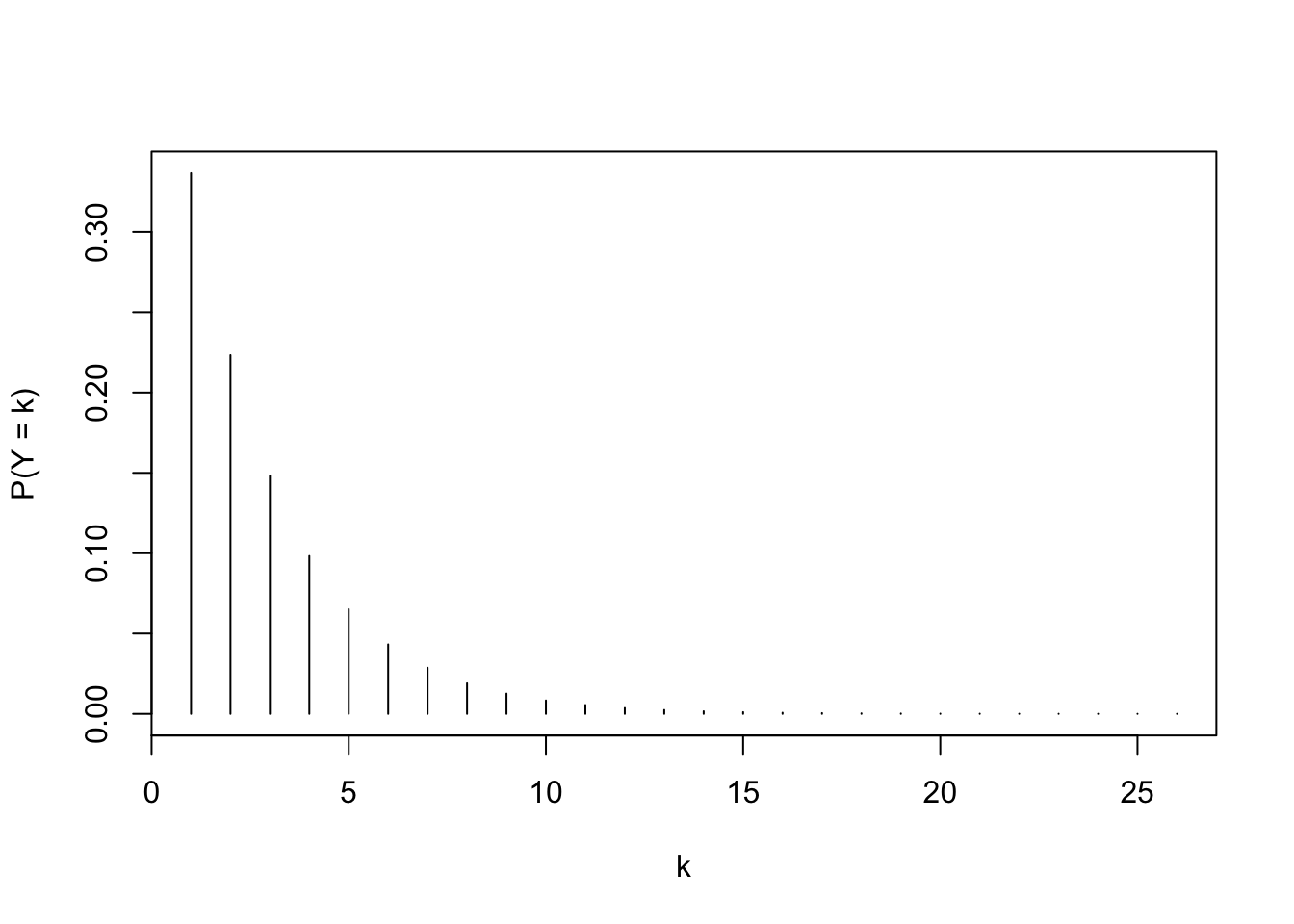
Let’s say that every day, I wake up, pour the coffee, do some lil’ granny stretches so that I don’t break a hip, and then swipe on the app until I’ve sent out my 25 likes for the day. Then I wait to see if any matches roll in. I do this day after day after day. Let \(Y\) be the number of days I have to wait through until I get at least one match.
What is the distribution of \(Y\)? Use R to plot its PMF.
Task 6
Let’s say I first downloaded the app on a Sunday. Use R to compute the probability that I get a match in the first week.
Solution
We want the probability that one of the first 7 trials is a success. So \(P(Y\leq 7)\):
pgeom(7 - 1, match_prob)[1] 0.9434099Task 7 (optional)
When you post your profile on a dating app, everyone in your area can see and swipe on it. If someone swipes right on you, the app will usually alert you to the fact that this happened, but they will charge you for the privilege of seeing who exactly it is. So let \(Z\) be the number of “likes” you receive in a given twenty-four hour period. We could model this using the Poisson distribution and say that \(Z\sim \text{Poisson}(\lambda)\). If we wish to model the likes received by some disgraced undesirable like James Corden, we might pick \(Z\sim \text{Poisson}(0.01)\), which has \(E(Z)=0.01\). Suffice it to say, not a tremendous number of likes rolling in for that guy, on average. If we wish to model the likes received by Taylor Swift, we might pick \(Z\sim\text{Poisson}(20,000,000)\). You get the idea.
For an ordinary person, perhaps \(Z\sim\text{Poisson}(5)\). Use R to compute the probability that such a person beats their average for the day.
Solution
We want \(P(Z>5)=1-P(Y\leq 5)\):
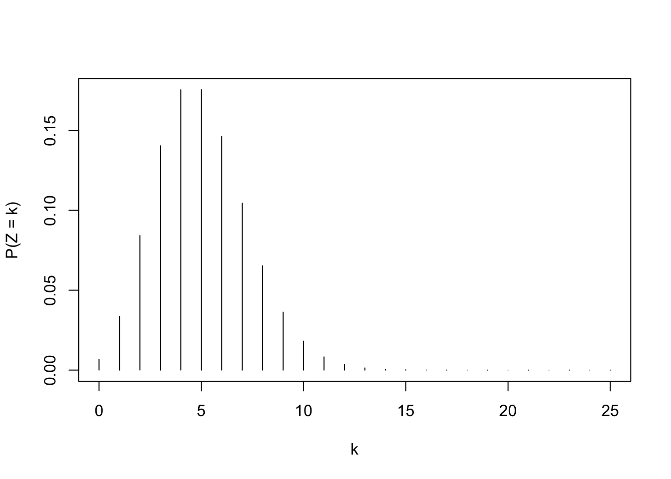
1 - ppois(5, lambda = 5)[1] 0.3840393Task 8 (optional)
Use R to plot the PMF of \(Z\).