Problem Set 6
Due Sunday November 9 at 5PM
Problem 0
Doodle a cute character that will cheer you on during this assignment.
Problem 1
Here is the cdf of an absolutely continuous random variable \(X\):
\[ F(x;\,\alpha,\,\theta) = \begin{cases} 1-\left(\frac{\theta}{x + \theta}\right)^\alpha & x >0 \\ 0 & \text{else}. \end{cases} \]
The parameters \(\alpha\) and \(\theta\) are just positive constants.
- Find the pdf of \(X\) and plot it for \(\alpha=1,\, 2,\, 3\) and \(\theta = 1\);
- Compute the median of \(X\);
- Compute \(E(X)\). Is it finite for all values of the parameters?
- Compute \(\textrm{var}(X)\). Is it finite for all values of the parameters?
- Fix \((\alpha,\,\theta) = (3,\, 100)\) and compute \(P(X > 75\,|\, X > 50)\).
Tip
On Problem Set 5 you met some cute alternatives for computing expected values, and they may be helpful here.
Problem 2
Quantum mechanics has a reputation for being an intimidating branch of theoretical physics, and JZ certainly doesn’t understand a ding dong thing about it. Even so, because we have studied some basic probability theory, the mathematics of quantum mechanics is more accessible than you might guess. Behold:
Imagine a single particle at the (sub)atomic level1. A particle’s quantum state encodes information about all of its measurable properties, such as position, momentum, spin, and energy. In quantum mechanics, measuring these properties is fundamentally probabilistic. Before measurement, the particle doesn’t have a single, definite position or momentum; it has only probabilities for the possible outcomes. The quantum state of a particle is fully characterized by its wave function, and the squared magnitude of the wave function is a probability density that describes the distribution of the particle’s position, or momentum, or whatever else you wish to study. Let’s explore this in a very simple example.
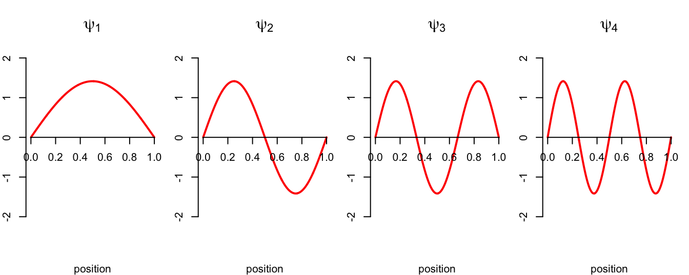
Consider a single, one-dimensional particle located somewhere in the interval \([0,\,L]\). The wave function associated with the particle’s quantum state is
\[ \psi_n(x) = \begin{cases} A\cdot\sin\left(\frac{n\pi}{L}x\right) & 0\leq x\leq L\\ 0 & \text{else}, \end{cases} \]
where \(A\geq 0\) is the amplitude, and \(n=1,\,2,\,3,\,...\) indexes the particle’s energy level. The higher the energy level, the more “excited” the particle is. Behold:
Because the particle does not have a definite position before measurement, we treat the position \(X_n\in[0,\,L]\) of the particle as a continuous random variable whose probability density function is \(f_n(x)=|\psi_n(x)|^2\).
- Compute the value of \(A\) that ensures that \(f_n\) is a valid pdf;
- Compute the cdf of the random variable \(X_n\) and plot it for various values of \(n\);
- What is the expected location of the particle?
- What is the probability that the particle is located at the midpoint of the interval?
- Let \(n=4\) and \(L=1\). What is the probability that the particle is located in the interval \([0.2, 0.3]\)?
- The parameter \(n=1,\,2,\,3,\,...\) indexes the energy level of the particle. The larger the value of \(n\), the more excited the particle is. If \(n\to\infty\), then the particle is, like, super stoked. What happens to the distribution of \(X_n\) as \(n\to\infty\)?
Problem 3
Let \(X\) be a discrete random variable with
| \(x\) | -1 | 3 | 7 |
|---|---|---|---|
| \(P(X=x)\) | 0.5 | 0.2 | 0.3 |
- Compute the mgf of \(X\).
- Compute the mean two ways: using the definition, and using the mgf. Confirm that you get the same answer.
- Compute the variance two ways: using the definition, and using the mgf. Confirm that you get the same answer.
Problem 4
- Compute the moment-generating function of the binomial distribution;
- Use the mgf to compute the mean;
- Use the mgf to compute the variance.
Note: we already know from lecture that the mean is \(np\) and the variance is \(np(1-p)\), so you know you did it right when you get the same answer.
Problem 5
Let \(X\) have density
\[ f_X(x) = \frac{1}{2} e^{-|x|},\quad x\in\mathbb{R}. \]
- What is the mgf of \(X\)?
- What is the mean?
- What is the variance?
Problem 6
On Lab 7, we learned how to derive the distribution of a transformation. This is an important technical skill that crops up often in mathematical probability, so let’s get our reps in:
- Let \(X\sim\text{Unif}(0,\,1)\), and find the range and density of \(Y=e^X\);
- Let \(X\sim\textrm{Unif}(0,\,1)\), and find the range and density of \(Y=\sqrt{X}\);
- Let \(X\sim\text{Unif}(0,\,1)\), and find the range and density of \(Y=X^2\);
- Let \(X\sim\text{Gamma}(a,\,b)\), and find the range and density of \(Y=1/X\);
- Let \(Z\sim\text{N}(0,\,1)\), and find the range and density of \(Z^2\).
Problem 7
Suppose \(X\) and \(Y\) are jointly absolutely continuous random variables with joint density
\[ f_{XY}(x,\,y)=xe^{-x(y+1)},\quad x,\,y>0. \]
- Find the marginal density of \(X\).
- Find the marginal density of \(Y\).
- Are \(X\) and \(Y\) independent?
- Find the conditional density of \(X\) given \(Y=y\).
- Find the conditional density of \(Y\) given \(X=x\).
Problem 8
Let \(X\) and \(Y\) be jointly absolutely continuous with density
\[ f_{XY}(x,\, y)=\frac{1}{\pi},\quad x^2+y^2\leq 1. \]
So \(X\) and \(Y\) jointly possess the uniform distribution on the unit disc.
- The joint density is a surface in three-dimensional space. Sketch what the joint density looks like.
- Compute the marginal densities of \(X\) and \(Y\).
- Are \(X\) and \(Y\) independent?
Problem 9
Consider a random pair \((X,\,Y)\) with a joint distribution given by this hierarchy:
\[ \begin{aligned} X &\sim \textrm{Beta}(a,\, b) \\ Y\mid X = x &\sim \textrm{Gamma}\left(a+b,\, \frac{c}{x}\right). \end{aligned} \]
- What is the joint range?
- What is the marginal density of \(Y\)?
- What is the conditional density of \(X\)?
New distribution!
If \(X\sim \textrm{Beta}(a,\, b)\), then \(\text{Range}(X)=(0,\,1)\) and the density is
\[ f(x)=\frac{\Gamma(a+b)}{\Gamma(a)\Gamma(b)}x^{a-1}(1-x)^{b-1},\quad0<x<1. \]
That’s new to you, so see if you can work with it.
Problem 10
Consider the joint distribution of random variables \(X\) and \(Y\), written in hierarchical form:
\[ \begin{aligned} X&\sim\textrm{Gamma}\left(\frac{d_2}{2},\, \frac{d_2}{2}\right)\\ Y\,|\, X = x&\sim\textrm{Gamma}\left(\frac{d_1}{2},\, \frac{d_1}{2}x\right).\\ \end{aligned} \]
Do some serious “massage and squint” to show that the marginal pdf of \(Y\) is
\[ f_Y(y)=\frac{\Gamma\left(\frac{d_1}{2}+\frac{d_2}{2}\right)}{\Gamma\left(\frac{d_1}{2}\right)\Gamma\left(\frac{d_2}{2}\right)}\left(\frac{d_1}{d_2}\right)^{\frac{d_1}{2}}y^{\frac{d_1}{2}-1}\left(1+\frac{d_1}{d_2}y\right)^{-\frac{d_1+d_2}{2}},\quad y>0. \]
This means that \(Y\) has the F-distribution.
Submission
You are free to compose your solutions for this problem set however you wish (scan or photograph written work, handwriting capture on a tablet device, LaTeX, Quarto, whatever) as long as the final product is a single PDF file. You must upload this to Gradescope and mark the pages associated with each problem.
Do not forget to include the following:
- For each problem, please acknowledge your collaborators;
- If a problem required you to code something, please include both the code and the output. “Including the code” can be as crude as a screenshot, but you might also use Quarto to get a nice lil’ pdf that you can merge with the rest of your submission.
Footnotes
If you’re like me, you cannot do this. Oh well.↩︎